One of the most famous models for quantum computation is the black-box model, in which one is given a black-box called oracle encoding a unitary operation. With this oracle one can probe the bits of an unknown bit string  (the paper uses the set
  instead of
  , which I will keep here) . The main aim of the model is to use the oracle to learn some property given by a Boolean function
  of the bit string
  , for example, its parity. One use of the oracle is usually referred as a query, and the number of queries a certain algorithm performs reflects its efficiency. Quite obviously, we want to minimize the number of queries. In more precise words, the bounded-error quantum query complexity of a Boolean function
  is denoted by
 ") and refers to the minimum number of queries a quantum algorithm must make on the worst-case input x in order to compute
and refers to the minimum number of queries a quantum algorithm must make on the worst-case input x in order to compute ") with probability
with probability  .
.
Looking at the model and the definition for the quantum query complexity, one might ask “but how can we find the query complexity of a certain function? Is there an easy way to do so?”. As usual in this kind of problem, finding the optimal performance of an algorithm for a certain problem or an useful lower bound for it is easier said than done. Nonetheless, there are some methods for tackling the problem of determining . There are two main methods for proving lower bounds, known as the polynomial method and the adversary method. In this post we shall talk about the first, the polynomial method, and how it was improved in the work of Arunachalam et al.
The polynomial method
The polynomial method is a lower bound method based on a connection between quantum query algorithms and, as the name suggests, polynomials. The connection comes from the fact that for every t-query quantum algorithm  that returns a random sign
 ") (i.e. ) on input , there exists a degree–
(i.e. ) on input , there exists a degree– polynomial
  such that
 ") equals the expected value of . From this it follows that if computes a Boolean function with probability at least , then the polynomial satisfies
equals the expected value of . From this it follows that if computes a Boolean function with probability at least , then the polynomial satisfies  - f(x)| \leq 2\epsilon") for every (the factor of
for every (the factor of  comes from the image being instead of ). Therefore we can see that the minimum degree of a polynomial that satisfies for every , called the approximate (polynomial) degree and denoted by
 ") , serves as a lower bound for the query complexity . Hence the problem of finding a lower bound for the query complexity is converted into the problem of lower bounding the degree of such polynomials.
, serves as a lower bound for the query complexity . Hence the problem of finding a lower bound for the query complexity is converted into the problem of lower bounding the degree of such polynomials.
Converse to the polynomial method
We now have a method for proving lower bounds for quantum query algorithms by using polynomials. A natural question that can arise is whether the polynomial method has a converse, that is, if a degree- polynomial leads to a  –query quantum algorithm. This would in turn imply a sufficient characterization of quantum query algorithms. Unfortunately, Ambainis showed in 2006 that this is not the case, by proving that for infinitely many
  , there is a function with
  \leq n^\alpha") and
and  \geq n^\beta") for some positive constants
for some positive constants  . Hence the approximate degree is not such a precise measure for quantum query complexity in most cases.
In the view of these negative results, the question that stays is, is there some refinement to the approximate polynomial that approximates ") up to a constant factor? Aaronson et al. tried to answer this question around 2016 by introducing a refined degree measure, called block-multilinear approximate polynomial degree and denoted by
up to a constant factor? Aaronson et al. tried to answer this question around 2016 by introducing a refined degree measure, called block-multilinear approximate polynomial degree and denoted by ") , which comes from polynomials with a so-called block-multilinear structure. This refined degree lies between and
, which comes from polynomials with a so-called block-multilinear structure. This refined degree lies between and ") , which leads to the question of how well that approximates . Once again, it was later shown that for infinitely many , there is a function with
, which leads to the question of how well that approximates . Once again, it was later shown that for infinitely many , there is a function with  = O(\sqrt{n})") and
and  = \Omega(n)") , ruling out the converse for the polynomial method based on the degree and leaving the question open until now, when it was answered by Arunachalam et al., who gave a new notion of polynomial degree that tightly characterizes quantum query complexity.
, ruling out the converse for the polynomial method based on the degree and leaving the question open until now, when it was answered by Arunachalam et al., who gave a new notion of polynomial degree that tightly characterizes quantum query complexity.
Characterization of quantum algorithms
In few words, it turns out that -query quantum algorithms can be fully characterized using the polynomial method if we restrict the set of degree- polynomials to forms that are completely bounded. A form is a homogeneous polynomial, that is, a polynomial whose non-zero terms all have the same degree, e.g.  is a form of degree . And the notion of completely bounded involves the idea of a very specific norm, the completely bounded norm (denoted by
  ), which was originally introduced in the general context of tensor products of operator spaces. But before we venture ourselves into this norm, which involves symmetric tensors and other norms, let us state the main result of the quantum query algorithms characterization.
Let ![\beta: \{-1,1\}^n \to [-1,1]](https://s0.wp.com/latex.php?latex=%5Cbeta%3A+%5C%7B-1%2C1%5C%7D%5En+%5Cto+%5B-1%2C1%5D&bg=ffffff&fg=000000&s=0 "\beta: \{-1,1\}^n \to [-1,1]") and a positive integer. Then, the following are equivalent.
and a positive integer. Then, the following are equivalent.
1. There exists a form of degree such that  and
and ) = \beta(x)") for every
for every  , where
  is the all-ones vector.
2. There exists a -query quantum algorithm that returns a random sign with expected value ") on input .
on input .
In short, if we find a form of degree which is completely bounded () and approximates a function that we are trying to solve, then there is a quantum algorithm which makes queries and solves the function. Hence we have a characterization of quantum algorithms in terms of forms that are completely bounded. But we still haven’t talked about the norm itself, which we should do now. It will involve a lot of definitions, some extra norms and a bit of C*-algebra, but fear not, we will go slowly.
The completely bounded norm
For  , we write
  . Any form of degree can be written as
 = \sum_{|\alpha| = t} c_{\alpha} x^\alpha") ,
,
where  are real coefficients. The first step towards the completely bounded norm of a form is to define the completely bounded norm of a tensor, and the tensor we use is the symmetric -tensor
  defined as
_\alpha = c_\alpha/|\{\alpha\}|!")
where  denotes the number of distinct elements in the set formed by the coordinates of
  .
.
The relevant norm of is given in terms of an infimum over decompositions of the form  , where
  is a permutation of the set
  and
and _\alpha = T^\sigma_{\sigma(\alpha)}") is the permuted element of the multilinear form
is the permuted element of the multilinear form  . So that the completely bounded norm of is kind of transferred to via the definition
 .
.
Just to recap, with the coefficients of the polynomial we define the symmetric -tensor , which is then decomposed into the sum of permuted tensor (multilinear form) . We then define the completely bounded norm of as the infimum of the sum of the completely bounded norm of such tensor, but now without permuting it. Of course, we haven’t yet defined the completely bounded norm of such tensor, that is, what is  ? We will explain it now.
The idea is to get a bunch of collections of  unitary matrices
 , U_2(i), \dotsc, U_t(i)") for
for  and consider the quantity
U_2(j)\dotsc U_t(k)\|") .
.
We multiply the unitaries from these collections and sum them using the tensor as weight, and then take the norm of the resulting quantity. But here we are using a different norm, the usual operator norm defined for a given operator as  . Finally, with these ingredients in hand, we can define the completely bounded norm for , which is just the supremum over the positive integer
  and the unitary matrices, that is,
U_2(j)\dotsc U_t(k)\| : d \in \mathbb{N}, d \times d \text{ unitary matrices } U_i\}") .
.
If we can obtain the supremum of such norm over the size of the unitary matrices and the unitary matrices themselves, then we obtain the completely bounded norm of the tensor , and from this we get the completely bounded norm of the associated form . Is there such a degree- form with that approximates the function we want to solve? If yes, then there is a -query quantum algorithm that solves .
The proof
Let us briefly explain the proof of the quantum algorithms characterization that we stated above. Their proof involves three main ingredients. The first one is a theorem by Christensen and Sinclair showing that the completely-boundedness of a multilinear form is equivalent to a nice decomposition of such multilinear form. In other words, for a multilinear form  , we have that
  if and only if we can write as
 = V_1\pi(x_1)V_2\pi(x_2)V_3\dotsc V_t\pi(x_t)V_{t+1}") , (1)
, (1)
where  are contractions (
 for every ) and
  are *-representations (linear maps that preserve multiplication operations,
  = \pi(x)\pi(y)") ).
).
The second ingredient gives an upper bound on the completely bounded norm of a certain linear map if it has a specific form. More specifically, if is a linear map such that  = U\pi(x)V") , where
, where  and
and  are also linear maps and
  is a *-representation, then
  .
.
The third ingredient is the famous Fundamental Factorization Theorem that “factorizes” a linear map in terms of other linear maps if its completely bounded norm is upper bounded by these linear maps. In other words, if is a linear map and exists other linear maps and such that  , then, for every matrix
  , we have
  = U^\ast(M\otimes I)V") .
.
With these ingredients, they proved an alternative decomposition of equation (1) which was later used to come up with a quantum circuit implementing the tensor and using queries, and then showed that this tensor matched the initial form . This alternative decomposition is
 = u^\ast U_1^\ast (\text{Diag}(x_1)\otimes I)V_1 \dotsc U_t^\ast (\text{Diag}(x_t)\otimes I)V_tv") , (2)
, (2)
where  are contractions,
  are unit vectors,
 ") is the diagonal matrix whose diagonal forms . The above decomposition is valid if, similarly to (1), .
is the diagonal matrix whose diagonal forms . The above decomposition is valid if, similarly to (1), .
We can see that the decomposition involves the operator intercalated by unitaries times. Having as the query operator, it is possible then to come up with a quantum circuit implementing the decomposition (2). If we look more closely, decomposition (2) has unit vectors on both the left and right sides, which looks like an expectation value. So what is going on is that decomposition (2) can be used to construct a quantum circuit whose expectation value matches , and hence the polynomial used to construct . We won’t get into much details, but we will leave the quantum circuit so that the reader can have a glimpse of what is going on.

In the above figure representing a quantum circuit that has as its expectation value, the registers C, Q, W denote control, query and workspace registers. The unitaries  are defined by
  , the unitaries
  have
have  and
and  as their first rows, where
  and
and  are isometries ( is an isometry iff
  for every ).
Application of the characterization: separation for quartic polynomials
A couple of years ago, in 2016, Aaronson et al. showed that the bounded norm (and also the completely bounded norm that we spent some time describing) is sufficient to characterize quadratic polynomials. More specifically, they showed that for every bounded quadratic polynomial , there exists a one-query quantum algorithm that returns a random sign with expectation ") on input , where
on input , where  is an absolute constant. This readily prompted the question of whether the same is valid for higher-degree polynomials, that is, if the bounded norm suffices to characterize quantum query algorithms.
As you might expect by now, the answer is no, since it is the completely bounded norm that suffices, and Arunachalam et al. used their characterization to give a counterexample for bounded quartic polynomials. What they showed is the existence of a bounded (not completely bounded) quartic polynomial p that for any two-query quantum algorithm whose expectation value is , one must have ") , thus showing that is not an absolute constant. The way they showed this is by using a random cubic form that is bounded, but whose completely bounded norm is
, thus showing that is not an absolute constant. The way they showed this is by using a random cubic form that is bounded, but whose completely bounded norm is ") and then embedded this form into a quartic form.
and then embedded this form into a quartic form.
Conclusions
The characterization they found is, in my opinion, apart from the obvious point that it answers the open question of the converse of the polynomial method, quite interesting in the sense that the set of polynomials we should look at is the ones that are bounded by a particular norm, the completely bounded norm. The interesting point is exactly this one, the connection between quantum query algorithms and the completely bounded norm that was first introduced in the general context of tensor products of operator spaces as mentioned before. The norm itself looks quite exotic and complicated, which is linked to a question that Scott Aaronson made at the end of Arunachalam’s talk in QIP 2019, “sure, we could define a particular norm as one that restricts the set of polynomials to the ones that admit a converse to the polynomial method”. Of course, such a norm would not be quite an interesting one. He carries on with something like “In what is this completely bounded norm different compared to that?”. If I remember correctly, Arunachalam gave an answer on the lines of the completely bounded norm appearing in a completely different context. But I still find it surprising that you would go through all the exotic definitions we mentioned above for the completely bounded norm and discover that it is what is needed for the converse of the polynomial method.
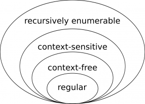
 is any language that can be constructed from:
 .
. .
. consisting of a single letter
  from the alphabet.
 ): ‘
): ‘ ‘.
‘. ): ‘either
  ): ‘zero or more repetitions of
  for union and omit some brackets. For example, to construct a regular language that recognises all words (over the Roman alphabet) that begin with ‘q’ and end with either ‘tum’ or ‘ta’, we could write the regular expression
 ") . In this case, the words ‘quantum’ and ‘quanta’ are contained in the regular language, but the words ‘classical’ and ‘quant’ are not. A more computationally motivated example is the regular expression for the
. In this case, the words ‘quantum’ and ‘quanta’ are contained in the regular language, but the words ‘classical’ and ‘quant’ are not. A more computationally motivated example is the regular expression for the  function over the binary alphabet
  , which we can write as
  (i.e. ‘a 1 surrounded by any number of any other characters’).
 , is
, is 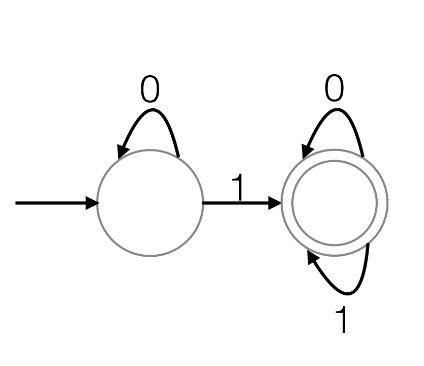
, \tilde{\Theta}(\sqrt{n})") , or
, or ") . Furthermore, each query upper bound results from an explicit quantum algorithm.
. Furthermore, each query upper bound results from an explicit quantum algorithm. — i.e. `something not in
  is equivalent to the language
  . The quantum query complexity of these languages is
 ") .
.") or
or ") queries for star-free regular languages extends to a variety of other settings by virtue of the fact that the star-free languages enjoy a number of equivalent characterisations. In particular, the characterisation of star-free languages as sentences in first-order logic over the natural numbers with the less-than relation shows that the algorithm for star-free languages is a nice generalisation of Grover’s algorithm. See Sections 1.3 and 4 of their paper for extra details and applications.
queries for star-free regular languages extends to a variety of other settings by virtue of the fact that the star-free languages enjoy a number of equivalent characterisations. In particular, the characterisation of star-free languages as sentences in first-order logic over the natural numbers with the less-than relation shows that the algorithm for star-free languages is a nice generalisation of Grover’s algorithm. See Sections 1.3 and 4 of their paper for extra details and applications. for
for ") is true if input symbol
is true if input symbol  is
is  .), it follows that all star-free languages that have quantum query complexity
") . Thus, another way to state the trichotomy is that (very roughly speaking) regular languages in
. Thus, another way to state the trichotomy is that (very roughly speaking) regular languages in 
") , regular languages in
, regular languages in ") ,
, ") , or
, or  many positions of
 ") queries. They also demonstrate that there exist context-free grammars which do not admit constant query property testers – showing that the results once again break down once we leave the regular languages.
queries. They also demonstrate that there exist context-free grammars which do not admit constant query property testers – showing that the results once again break down once we leave the regular languages.") .
.![c \in [1/2, 1]](https://s0.wp.com/latex.php?latex=c+%5Cin+%5B1%2F2%2C+1%5D&bg=ffffff&fg=000000&s=0 "c \in [1/2, 1]") , there exists some context-free language with quantum query complexity approaching
, there exists some context-free language with quantum query complexity approaching ") . They conjecture that no context-free language will have quantum query complexity that lies strictly between constant or
. They conjecture that no context-free language will have quantum query complexity that lies strictly between constant or  , but leave this open.
 ). Then our task is to determine whether there is an occurrence of
  at an even position (belongs to the language
 ^*01\Sigma^*") ). As the authors point out, we can use binary search to decide membership in only
). As the authors point out, we can use binary search to decide membership in only )") ,
, )") , or
, or )") .
. which can take the form
  where the
  are Hermitian operators. The type of parameters and operators depend on the device that is being targeted and
  is an easy-to-prepare initial state.
") you wish to minimise (or maximise) where
you wish to minimise (or maximise) where  = \langle\theta|H|\theta\rangle") and
and  is some Hermitian observable (for example corresponding to a physical Hamiltonian). Due to the randomness of quantum measurements, many preparations and measurements of
  that will minimise
  = \langle\theta|H|\theta\rangle = \sum_{i=1}^m \alpha_i\langle\theta|P_i|\theta\rangle")
 are tensor products of Pauli operators. Then to carry out the optimisation, derivative-free methods such as Nelder-Mead can be used. However, if one wishes to use derivative-based methods such as BFGS or the conjugate gradient method, we need an estimate of the gradient
 ") . A numerical way to do this is by finite-differencing which only requires measurements of
. A numerical way to do this is by finite-differencing which only requires measurements of  ,
,
 - f(\theta - \epsilon \hat{e}_i))")
 is the unit vector along the
  component. Each time
  is evaluated with different parameters, which can be done in low-depth, many repeat measurements are required.
 where the unitary
  and for
  the sequence
  is defined as
  . Therefore,
  = \langle\theta|H|\theta\rangle = \langle\psi|U^\dagger_{1:p}HU_{1:p}|\psi\rangle") . This can be differentiated via the chain rule to find:
. This can be differentiated via the chain rule to find:
:p} HU_{1:p}|\psi\rangle.")
 and writing the Pauli decomposition of
 } Q_k^{(j)}") where
where }") are products of Pauli operators, the derivative can be rewritten as
are products of Pauli operators, the derivative can be rewritten as
}\alpha_l \text{Im} \langle\psi|U^\dagger_{1:j} Q_k^{(j)} U^\dagger_{(j+1):p} P_l U_{1:p}|\psi\rangle.")
} U^\dagger_{(j+1):p} P_l U_{1:p}|\psi\rangle") is:
is: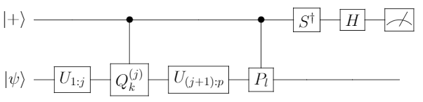
 encoding
  , parameters
  and a set
  containing integers
  . The black box then prepares the state
  performs a zeroth-order measurement estimating
  . The query cost of this model is the number of Pauli operators measured.
 -strongly convex
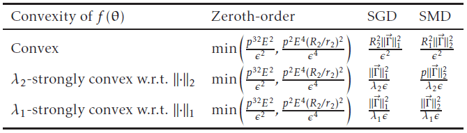
 and
and  are parameters related to the Pauli expansion of
  are balls in the convex region we are optimising over. It is clear that SGD and SMD will typically require less measurements to converge to the minimum compared to zeroth-order, but whether SGD outperforms SMD (or vice versa) depends on the problem at hand.
 -qubit Hamiltonians defined as the set
 }_v : \forall v \in \{-1,1\}^n\}") where
where  = \sqrt{\frac{45\epsilon}{n}}") and
and![H^\delta_v = -\sum_{i=1}^n \left[\text{sin}\left(\frac{\pi}{4} + v_i \delta\right)X_i + \text{cos}\left(\frac{\pi}{4} + v_i\delta\right)Z_i \right].](https://s0.wp.com/latex.php?latex=H%5E%5Cdelta_v+%3D+-%5Csum_%7Bi%3D1%7D%5En+%5Cleft%5B%5Ctext%7Bsin%7D%5Cleft%28%5Cfrac%7B%5Cpi%7D%7B4%7D+%2B+v_i+%5Cdelta%5Cright%29X_i+%2B+%5Ctext%7Bcos%7D%5Cleft%28%5Cfrac%7B%5Cpi%7D%7B4%7D+%2B+v_i%5Cdelta%5Cright%29Z_i+%5Cright%5D.+&bg=ffffff&fg=000000&s=1 "H^\delta_v = -\sum_{i=1}^n \left[\text{sin}\left(\frac{\pi}{4} + v_i \delta\right)X_i + \text{cos}\left(\frac{\pi}{4} + v_i\delta\right)Z_i \right].")
 are perturbations about
 ") where
where  is the strength and
  the direction of the perturbation. We wish to know how many measurements are needed to reach the ground state of
  . This problem is trivial (the lowest eigenvalue and it’s associated eigenvector can be written down directly) which is why the black-box formulation is necessary to hide the problem. The resulting upper and lower query complexity bounds for optimising the family
  is found to be:
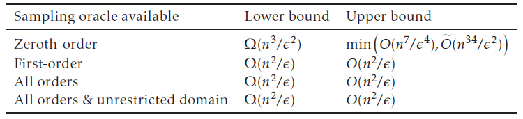
Y_j/2} \right)|0\rangle^{\otimes n}")
 plane. The corresponding objective function is then
  = -\sum_{i=1}^n \text{cos}(\theta_i - v_i\delta)") which is strongly convex near the optimum and so stochastic gradient descent performs well here. Note that making higher-order queries is unnecessary in this case as the optimal bounds can be achieved with just first-order.
which is strongly convex near the optimum and so stochastic gradient descent performs well here. Note that making higher-order queries is unnecessary in this case as the optimal bounds can be achieved with just first-order.