With the growing popularity of hybrid quantum-classical algorithms as a way of potentially achieving a quantum advantage on Noisy Intermediate-Scale Quantum (NISQ) devices, there were a number of talks on this topic at this year’s QIP conference in Boulder, Colorado. One of the talks that I found the most interesting was given by John Napp from MIT on how “Low-depth gradient measurements can improve convergence in variational hybrid quantum-classical algorithms” based on work done with Aram Harrow (https://arxiv.org/abs/1901.05374).
What are variational hybrid quantum-classical algorithms?
They are a class of optimisation algorithms in which the quantum and classical computer work closely together. Most variational algorithms follow a simple structure:
- Prepare a parameterised quantum state
which can take the form
where the
are Hermitian operators. The type of parameters and operators depend on the device that is being targeted and
is an easy-to-prepare initial state.
- Carry out measurements to determine information about the classical objective function
you wish to minimise (or maximise) where
and
is some Hermitian observable (for example corresponding to a physical Hamiltonian). Due to the randomness of quantum measurements, many preparations and measurements of
- Use a classical optimisation method to determine a new value for
that will minimise
- Repeat steps 1-3 until the optimiser converges.
Examples of this type of algorithm are the variational quantum eigensolver (VQE) used to calculate ground states of Hamiltonians and the quantum approximate optimisation algorithm (QAOA) for combinatoric optimisation problems.
Gradient measurements
To obtain information about the objective function
 = \langle\theta|H|\theta\rangle = \sum_{i=1}^m \alpha_i\langle\theta|P_i|\theta\rangle")
where 
")


 - f(\theta - \epsilon \hat{e}_i))")
where 


An alternative method is to take measurements that correspond directly to estimating the gradient
For the rest of this post, the term zeroth-order will refer to taking measurements corresponding to the objective function. First-order will refer to algorithms which make an analytic gradient measurement (and this can generalise to kth-order where the kth derivatives are measured). It is clear how zeroth-order measurements are made – by measuring the Pauli operators
The state 


 = \langle\theta|H|\theta\rangle = \langle\psi|U^\dagger_{1:p}HU_{1:p}|\psi\rangle")

:p} HU_{1:p}|\psi\rangle.")
Recalling that 
} Q_k^{(j)}")
}")

}\alpha_l \text{Im} \langle\psi|U^\dagger_{1:j} Q_k^{(j)} U^\dagger_{(j+1):p} P_l U_{1:p}|\psi\rangle.")
This can then be estimated using a general Hadamard test which is used to estimate real (or imaginary) parts of expected values. The circuit that yields an unbiased estimator for } U^\dagger_{(j+1):p} P_l U_{1:p}|\psi\rangle")
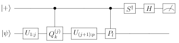
Measuring every term in the expansion is unnecessary to estimate
Black-box formulation
To quantify how complex an optimisation problem is, the function to be optimised
In this black-box model, the classical optimisation loop is given an oracle 


How many measurements are sufficient to converge to a local minimum?
Imagine now that we restrict to a convex region of the parameter space on which the objective function is also convex. We would like to know the upper bounds for the query complexity when optimising
In the paper, results from classical convex optimisation theory are used to compare a zeroth-order algorithm with stochastic gradient descent (SGD) and stochastic mirror descent (SMD, a generalisation of SGD to non-Euclidean spaces). For convex and 
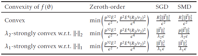
Here 


It is important to note that these are the best theoretical bounds, for some derivative-free algorithms (such as those based on trust regions) it can be hard to prove good upper bounds and guarantees of convergence. However they can perform very well in practice and so zeroth-order could still potentially outperform SGD and SMD.
Can first-order improve over zeroth-order measurements?
To answer this question, a toy problem was studied. Consider a class of 1-local 
}_v : \forall v \in \{-1,1\}^n\}")
 = \sqrt{\frac{45\epsilon}{n}}")
![H^\delta_v = -\sum_{i=1}^n \left[\text{sin}\left(\frac{\pi}{4} + v_i \delta\right)X_i + \text{cos}\left(\frac{\pi}{4} + v_i\delta\right)Z_i \right].](https://s0.wp.com/latex.php?latex=H%5E%5Cdelta_v+%3D+-%5Csum_%7Bi%3D1%7D%5En+%5Cleft%5B%5Ctext%7Bsin%7D%5Cleft%28%5Cfrac%7B%5Cpi%7D%7B4%7D+%2B+v_i+%5Cdelta%5Cright%29X_i+%2B+%5Ctext%7Bcos%7D%5Cleft%28%5Cfrac%7B%5Cpi%7D%7B4%7D+%2B+v_i%5Cdelta%5Cright%29Z_i+%5Cright%5D.+&bg=ffffff&fg=000000&s=1 "H^\delta_v = -\sum_{i=1}^n \left[\text{sin}\left(\frac{\pi}{4} + v_i \delta\right)X_i + \text{cos}\left(\frac{\pi}{4} + v_i\delta\right)Z_i \right].")
These 
")


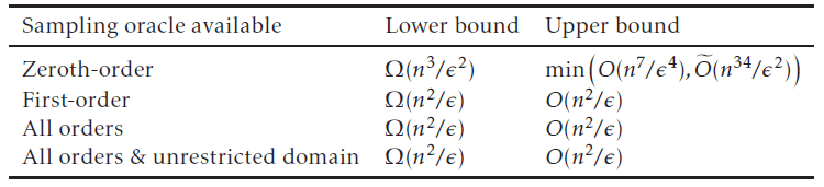
The proof of the lower bound is too complicated to explain here. Proving the upper bound, in particular for first-order, is simpler and relies on using a good parameterisation
Y_j/2} \right)|0\rangle^{\otimes n}")
in our optimisation algorithm. 
 = -\sum_{i=1}^n \text{cos}(\theta_i - v_i\delta)")
Conclusion
Ultimately Harrow and Napp have shown that there are cases in which taking analytic gradient measurements in variational algorithms for use in stochastic gradient/mirror descent optimisation routines (compared to derivative-free methods) could help with convergence. It would be interesting to see what happens with more complicated problems and if more general kth-order measurements will provide benefits over first-order. Another extension that is mentioned in the paper is to see what the impact of noisy qubits and gates is on the convergence of the optimisation problem.
I personally am most eager to see how these results will hold up in practice. For example, it would be interesting to see a simple simulation performed for the toy problem comparing zeroth-order optimisers with those that take advantage of analytic gradient measurements.